|
There are excellent blog posts written that visually break down the distinct layers of a convolutional neural network (CNN) and explain what is happening at each step. Great images like the one below, show us how a fully developed CNN is put together. 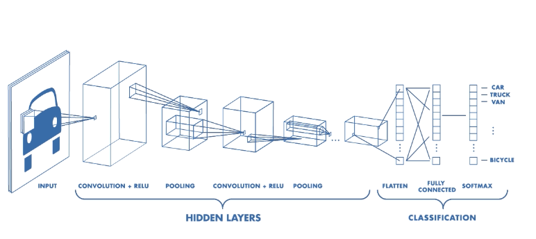 For this post, I will be explaining the layers of a CNN and writing a sort of glossary to a final CNN for an image classification model using the MNIST Fashion dataset. Rather then explaining the visual architecture of a CNN, I will be showing you my final model, which showed a 92% test accuracy and a 93% validation accuracy, and explaining the layers you see from a code perspective. For my full notebook, please visit my GitHub notebook Now, here is what my final model looks like: 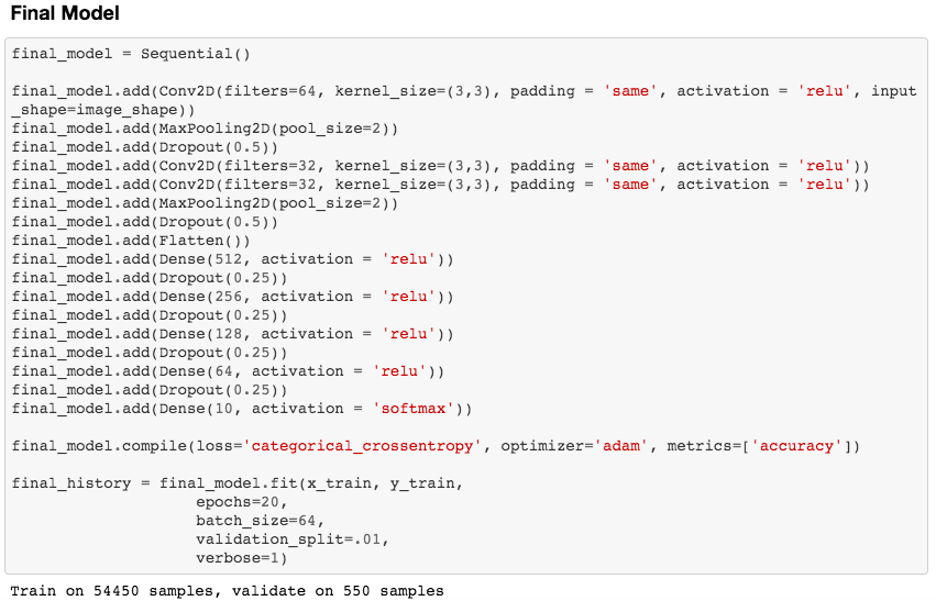 What will follow will be a glossary, not in alphabetical order, but in order as the parameters appear in my model. 1. What type of model? Sequential() - Generally, when building a model from scratch in which you choose what layers go on top of what layers, you use a sequential model. Using a sequential model is like making a pizza at home. The second option would be to construct a CNN using a functional API, or ordering out, in doing so, having more options for toppings and all those appetizers you just can't seem to make in your own kitchen. Functional API's give the data scientist more flexibility than the rigid, built from scratch, sequential model. For more on the differences between sequential models and functional API's click here. 2. The Convolutional Layer Conv2d() - This is the first convolutional layer. This is where a filter (shown in blue) strides across the image you are feeding the network. It performs what is basically the chain-rule and computing one number to represent, in this case, a 3 x 3 pixel section of the image and translating it to the purple square. This gives that section of the image one number. Once each purple square in the image below is filled in, you have a feature map. filters 64 - The first parameter in my Conv2d layer is filters = 64. This number refers to the number of actual filters I want to pass over my images. Each filter is randomly initialized and searching each image, learning about different features as it goes along. One filter may focus more on edges and lines. Another feature might be randomly initialized to focus on shapes. This means that within that first convolutional layer, we have 64 different filters passing over each image in our dataset. This number decreases to 32 in later layers. More can be uncovered here. kernel_size - this is simply the size of the filter that is being passed over the image. In most cases, we use a 3 x 3 filter or, kernel size. 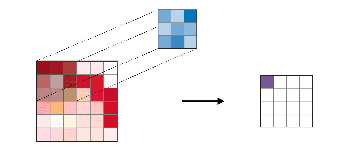 padding - In the image above, the dark red pixel in the top left corner will only be passed over by the filter 1 time. However, the orange looking pixel near the center of the image will be passed over much more than one time. This gives the orange pixel more weight when training. Therefore, padding sets a border of pixels with 0's around the image you are training on so that each individual pixel will have the same amount of time in the filter. The 'same' parameter simply allows the border of 0's to be the right size so the filter can move smoothly over the image and collect an equal amount of information about each pixel. activation - The final step in a convolutional layer is to send the inputs through a activation function. The ReLu activation function takes in a continuous variable input and outputs the same number, unless the input number is negative or 0. If that is the case, it will return a zero, giving it less importance and less likelihood of that neuron firing. This allows each node to have a number which in turn decides whether or not that node will fire when training on or testing an image. The continuous variable is passed through the activation function in order to decide whether or not to 'activate' that specific layer. 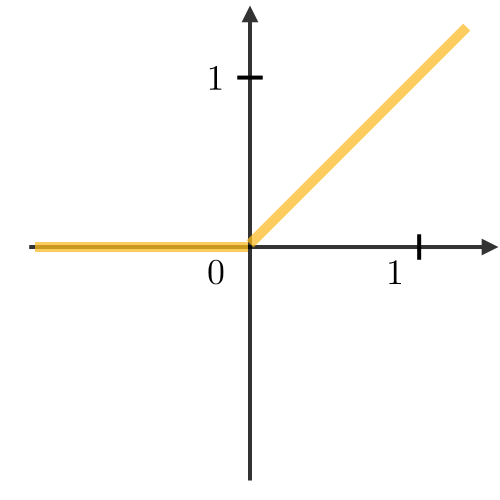 ReLu Activation Function https://stanford.edu/~shervine/teaching/cs-230/cheatsheet-convolutional-neural-networks 3. Max Pooling After our convolutional layer, we should have a series of filtered pixels, or the box above filled with purple boxes, or what we would call the feature map. Each image passing through each filter will have it's own feature map. This feature map needs to be downsized. Bring in the pooling layer. In my case, Max Pooling takes the maximum number in a 2 x 2 frame and creates what is essentially a new, smaller, more refined feature map. How do we know it is a 2 x 2 frame? Well you can see that in my model the pool_size parameter has been set to a 2, creating a nice 2 x 2 down-sizer to scan across our feature map. Here is a great place to learn more and another big shout out to the excellent tutorials written on Machine Learning Mastery. 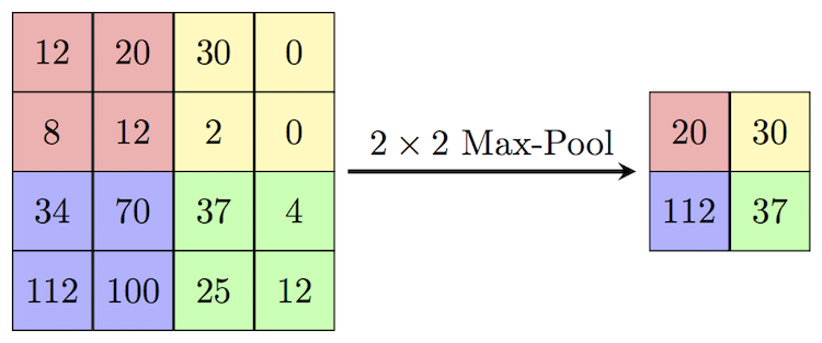 4. Dropout When training a model the CNN will go through forward and backward propagation. The dropout method is one that randomly drops out or silences a selection of nodes. Why do this? It helps with overfitting of course. When certain trained nodes are randomly dropped out, the nodes that are left have to pick up the extra work load. This leads to the network becoming less sensitive to individual nodes and more diverse, leading to a less likely situation where over fitting and relying on certain nodes to over train could occur. You'll notice that I have a few dropout layers in my model, each dropping out 25% of the nodes in my network. Here is a great resource that explains more. 5. Flatten This is a simple step that takes a feature map or a pooled feature map and converts the digits into a single column array to prep the data before it enters the dense layer. 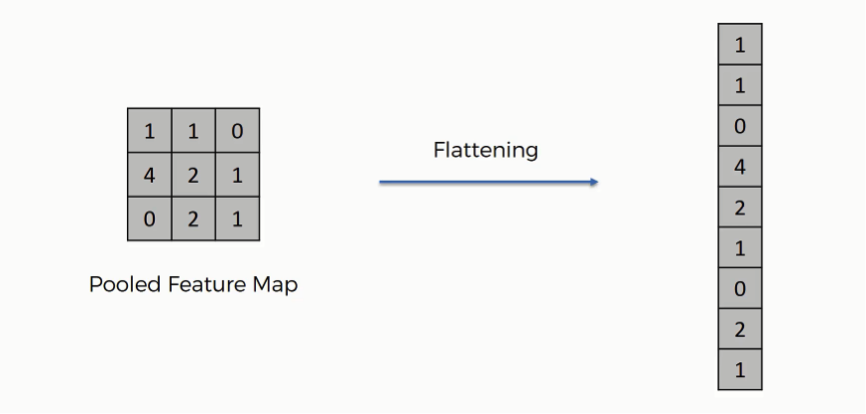 6. Dense layer This final layer uses a soft max activation function to generate 10 outcomes or our 10 categories for classifying our data. This will be the final, spit out a number type of layer. It creates a vector of probabilities as to what the image should most likely be classified as. Conclusion These neural networks can be very complicated by their very nature. Breaking down each layer and then further breaking down the parameters involved in those layers can be a very helpful approach to better understanding the overall network. I hope this helped give more insight to each of those things. Sources:
https://towardsdatascience.com/the-4-convolutional-neural-network-models-that-can-classify-your-fashion-images-9fe7f3e5399d https://adventuresinmachinelearning.com/keras-tutorial-cnn-11-lines/ https://forums.fast.ai/t/dense-vs-convolutional-vs-fully-connected-layers/191/3 https://adventuresinmachinelearning.com/keras-tutorial-cnn-11-lines/ https://www.superdatascience.com/blogs/convolutional-neural-networks-cnn-step-3-flattening https://towardsdatascience.com/activation-functions-and-its-types-which-is-better-a9a5310cc8f https://stats.stackexchange.com/questions/296679/what-does-kernel-size-mean/339265 https://machinelearningmastery.com/dropout-regularization-deep-learning-models-keras/ https://dashee87.github.io/deep%20learning/visualising-activation-functions-in-neural-networks/ https://stanford.edu/~shervine/teaching/cs-230/cheatsheet-convolutional-neural-networks
0 Comments
|
 RSS Feed
